3  Characterisation

This chapter is about characterising the biquad filter with the help of computational software like python and and comparing that with ideal circuit simulations. The comparison between a mathematical approach and a basic circuit implementation, gives a first impression if the filter is operational.

3.1 Behauvioural Analysis and macro modelling

The behauvioural analysis is done through macro modelling the universal biquad filter as a system. The system can be described with transfer functions and modelled with python.

3.1.1 Transfer Functions and frequency response

The ASLK PRO Manual (Rao and Ravikumar 2012) provides the transfer functions of the four filter outputs: low pass, high pass, band pass, and band stop. The transfer functions are adaptations of the general second order transfer function as seen in Equation 2.1. (Razavi 2018)

In the following transfer function the input and output voltage are referenced according to Figure 2.1. The sections only contain their specific transfer function and frequency response.

Low pass

The output if the low pass filter is marked in the circuit (Figure 2.1) as \(LPF\) and corresponds to \(V_{03}\) in the transfer function Equation 3.1.

\[ \frac{V_{03}}{V_i} = \frac{H_0}{\left( 1 + \frac{s}{\omega_0 Q} + \frac{s^2}{\omega_0^2} \right)} \tag{3.1}\]

Figure 3.1 shows the amplitude and phase response of the low pass filter. The required frequency \(f_0 = 1\,kHz\) and quality factor \(Q = 10\) recognizable in the bode plot. As the dc-gain was chosen to be \(H_0 = 1\), the low pass filter has a amplitude amplification of 1 in the lower frequencies.

Listing 3.1

# Behavioral Analysis Biquad Filter

import numpy as np
import matplotlib.pyplot as plt

# Initial values
f0 = 1e3  # Resonance frequency in Hz
w0 = 2 * np.pi * f0  # Angular frequency in rad/s
Q = 10  # Quality factor
H0 = 1  # Play around with this later

# Logarithmic frequency axis
frequencies = np.logspace(2, 4, 10000)  # Frequency from 10^2 to 10^4 Hz
s = 1j * 2 * np.pi * frequencies  # Laplace-Variable s = jω

############################################
# Transfer functions of Active Filters
############################################

### Numerator
# Low Pass Filter
b_lp = H0

# High Pass Filter
b_hp = (H0 * (s**2 / w0**2))

# Band Pass Filter
b_bp = (-H0 * (s / w0))

# Band Stop Filter
b_bs = -((1 + (s**2 / (w0**2))) * H0)

# Denominator -> for all filters the same
a0 = 1
a1 = (s / (w0 * Q))
a2 = (s**2 / (w0**2))

den = a0 + a1 + a2

############################################
# Calculation of the transfer functions H(s)
############################################
Hs_lp = b_lp / den
Hs_hp = b_hp / den
Hs_bp = b_bp / den
Hs_bs = b_bs / den

# Bode Diagram
fig, axs = plt.subplots(2)
#fig.suptitle("frequency response of biquad filter")

# Low Pass Filter
axs[0].semilogx(frequencies, 20 * np.log10(np.abs(Hs_lp)), label='low pass')
axs[1].semilogx(frequencies, np.unwrap(np.angle(Hs_lp)) * (180 / np.pi), label='low pass')
'''
# High Pass Filter
axs[0].semilogx(frequencies, 20 * np.log10(np.abs(Hs_hp)), label='high pass')
axs[1].semilogx(frequencies, np.unwrap(np.angle(Hs_hp)) * (180 / np.pi), label='high pass')

# Band Pass Filter
axs[0].semilogx(frequencies, 20 * np.log10(np.abs(Hs_bp)), label='band pass')
axs[1].semilogx(frequencies, np.unwrap(np.angle(Hs_bp)) * (180 / np.pi), label='band pass')

# Band Stop Filter
axs[0].semilogx(frequencies, 20 * np.log10(np.abs(Hs_bs)), label='band stop')
axs[1].semilogx(frequencies, (np.angle(Hs_bs)) * (180 / np.pi), label='band stop')
'''
#axs[0].title("amplitude response")
axs[0].set_xlabel("frequency/Hz")
axs[0].set_ylabel("amplitude/dB")
axs[0].set_ylim(-50, 25)
axs[0].grid(True, which="both", ls="--")
#axs[0].legend(loc=1)

#axs[1].title("phase response")
axs[1].set_xlabel("frequency/Hz")
axs[1].set_ylabel("phase/deg")
axs[1].grid(True, which="both", ls="--")
#axs[1].legend()

plt.tight_layout()
#plt.show()

plt.savefig("../images/sec_characterisation/freqResponseLowpass.png", format="png",dpi=1000)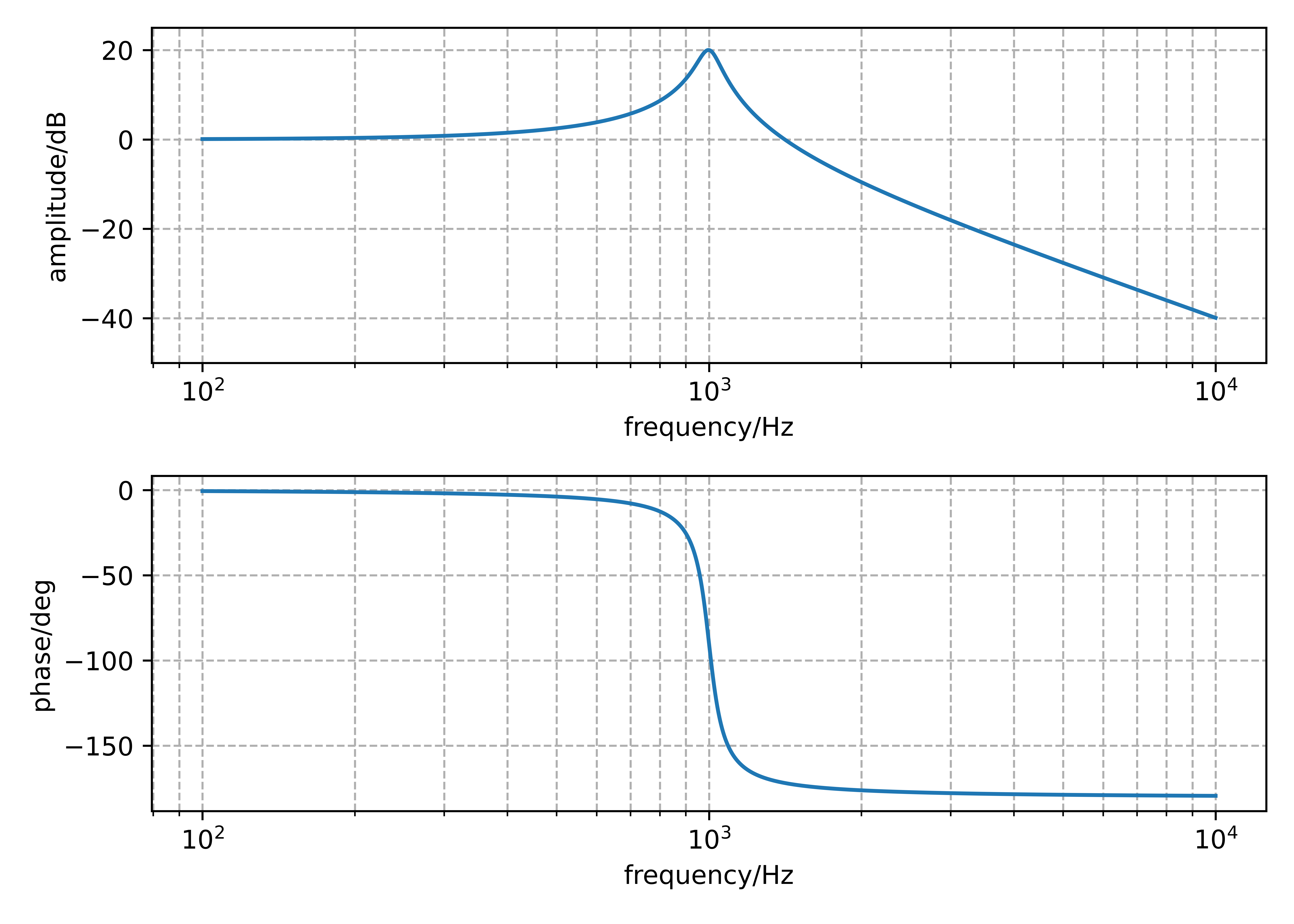

Figure 3.1: Frequency response of the low pass filter

With knowing the dc gain \(H_0 = 1\) and quality factot \(Q = 10\), the amplitude of the peak can be calculated as seen in Equation 2.3. Expression the value in dB, gives peak amplitude of \(A_{peak,dB} = 20.002\,dB\) which corresponds to the peak value seen in Figure 3.1.

High pass

The output if the high pass filter is marked in the circuit (Figure 2.1) as \(HPF\) and corresponds to \(V_{01}\) in the transfer function Equation 3.2.

\[ \frac{V_{01}}{V_i} = \frac{\left( H_0 \cdot \frac{s^2}{\omega_0^2} \right)}{\left( 1 + \frac{s}{\omega_0 Q} + \frac{s^2}{\omega_0^2} \right)} \tag{3.2}\]

Figure 3.2 shows the amplitude and phase response of the high pass filter. The required frequency \(f_0 = 1\,kHz\) and quality factor \(Q = 10\) recognizable in the bode plot. As the dc-gain was chosen to be \(H_0 = 1\), the low pass filter has a amplitude amplification of 1 in the higher frequencies.

Listing 3.2

# Behavioral Analysis Biquad Filter

import numpy as np
import matplotlib.pyplot as plt

# Initial values
f0 = 1e3  # Resonance frequency in Hz
w0 = 2 * np.pi * f0  # Angular frequency in rad/s
Q = 10  # Quality factor
H0 = 1  # Play around with this later

# Logarithmic frequency axis
frequencies = np.logspace(2, 4, 10000)  # Frequency from 10^2 to 10^4 Hz
s = 1j * 2 * np.pi * frequencies  # Laplace-Variable s = jω

############################################
# Transfer functions of Active Filters
############################################

### Numerator
# Low Pass Filter
b_lp = H0

# High Pass Filter
b_hp = (H0 * (s**2 / w0**2))

# Band Pass Filter
b_bp = (-H0 * (s / w0))

# Band Stop Filter
b_bs = -((1 + (s**2 / (w0**2))) * H0)

# Denominator -> for all filters the same
a0 = 1
a1 = (s / (w0 * Q))
a2 = (s**2 / (w0**2))

den = a0 + a1 + a2

############################################
# Calculation of the transfer functions H(s)
############################################
Hs_lp = b_lp / den
Hs_hp = b_hp / den
Hs_bp = b_bp / den
Hs_bs = b_bs / den

# Bode Diagram
fig, axs = plt.subplots(2)
#fig.suptitle("frequency response of biquad filter")

# Low Pass Filter
#axs[0].semilogx(frequencies, 20 * np.log10(np.abs(Hs_lp)), label='low pass')
#axs[1].semilogx(frequencies, np.unwrap(np.angle(Hs_lp)) * (180 / np.pi), label='low pass')

# High Pass Filter
axs[0].semilogx(frequencies, 20 * np.log10(np.abs(Hs_hp)), label='high pass')
axs[1].semilogx(frequencies, np.unwrap(np.angle(Hs_hp)) * (180 / np.pi), label='high pass')
'''
# Band Pass Filter
axs[0].semilogx(frequencies, 20 * np.log10(np.abs(Hs_bp)), label='band pass')
axs[1].semilogx(frequencies, np.unwrap(np.angle(Hs_bp)) * (180 / np.pi), label='band pass')

# Band Stop Filter
axs[0].semilogx(frequencies, 20 * np.log10(np.abs(Hs_bs)), label='band stop')
axs[1].semilogx(frequencies, (np.angle(Hs_bs)) * (180 / np.pi), label='band stop')
'''
#axs[0].title("amplitude response")
axs[0].set_xlabel("frequency/Hz")
axs[0].set_ylabel("amplitude/dB")
axs[0].set_ylim(-50, 25)
axs[0].grid(True, which="both", ls="--")
#axs[0].legend(loc=1)

#axs[1].title("phase response")
axs[1].set_xlabel("frequency/Hz")
axs[1].set_ylabel("phase/deg")
axs[1].grid(True, which="both", ls="--")
#axs[1].legend()

plt.tight_layout()
#plt.show()

plt.savefig("../images/sec_characterisation/freqResponseHighpass.png", format="png", dpi=1000)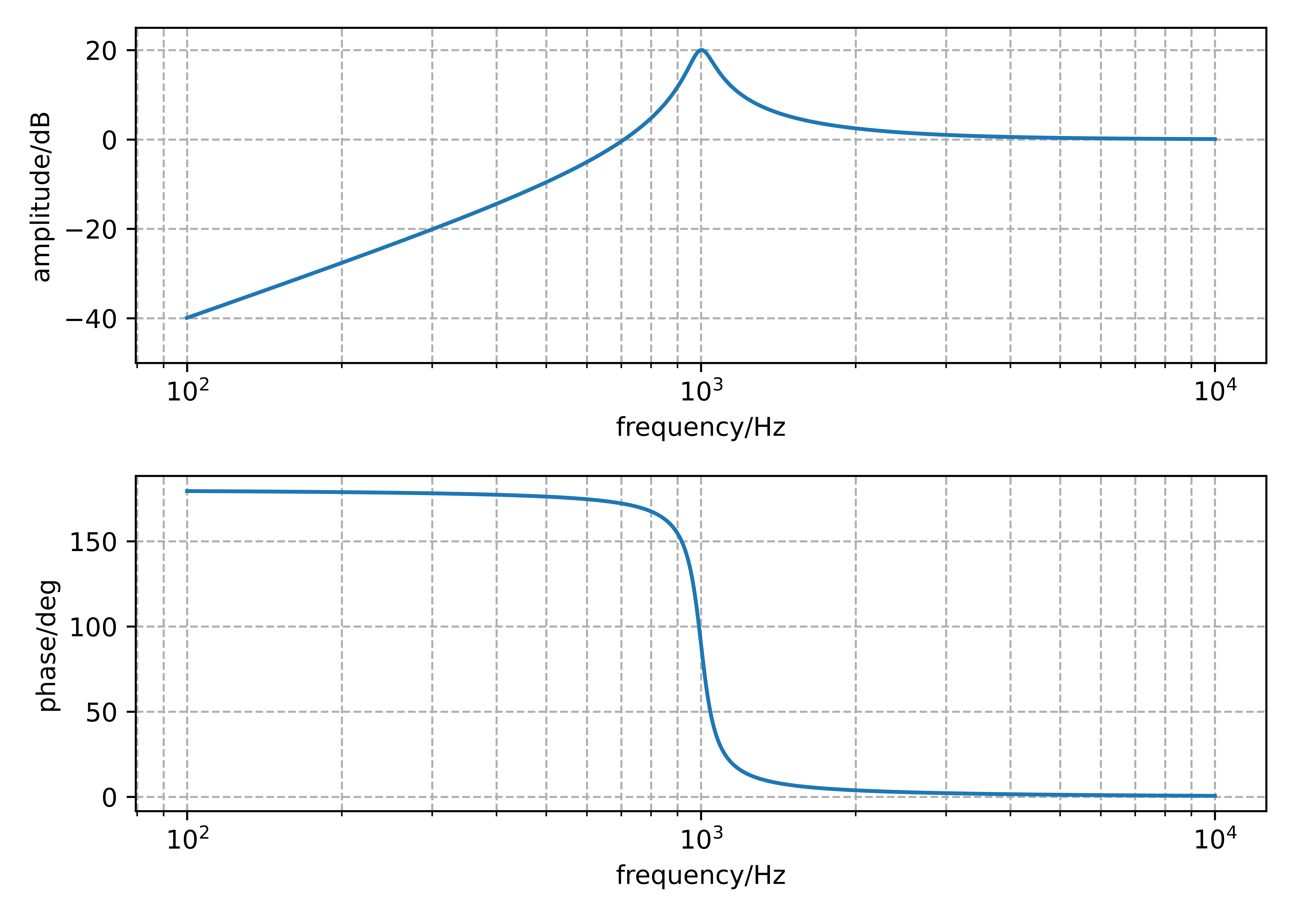

Figure 3.2: Frequency response of the high pass filter

Band pass

The output for the band pass filter is marked as \(BPF\) in Figure 2.1. This denotes the point that is referenced in Equation 3.3 as \(V_{02}\).

\[ \frac{V_{02}}{V_i} = \frac{\left( - H_0 \cdot \frac{s}{\omega_0} \right)}{\left( 1 + \frac{s}{\omega_0 Q} + \frac{s^2}{\omega_0^2} \right)} \tag{3.3}\]

The band pass shown in Figure 3.3 has its center frequency at \(1\,kHz\) as set in the requirements. Similarly to the low pass filter in Figure 3.1 and the high pass filter in Figure 3.2 the amplitude response peaks at this frequency, with its peak influenced by the quality factor.

Listing 3.3

# Behavioral Analysis Biquad Filter

import numpy as np
import matplotlib.pyplot as plt

# Initial values
f0 = 1e3  # Resonance frequency in Hz
w0 = 2 * np.pi * f0  # Angular frequency in rad/s
Q = 10  # Quality factor
H0 = 1  # Play around with this later

# Logarithmic frequency axis
frequencies = np.logspace(2, 4, 10000)  # Frequency from 10^2 to 10^4 Hz
s = 1j * 2 * np.pi * frequencies  # Laplace-Variable s = jω

############################################
# Transfer functions of Active Filters
############################################

### Numerator
# Low Pass Filter
b_lp = H0

# High Pass Filter
b_hp = (H0 * (s**2 / w0**2))

# Band Pass Filter
b_bp = (-H0 * (s / w0))

# Band Stop Filter
b_bs = -((1 + (s**2 / (w0**2))) * H0)

# Denominator -> for all filters the same
a0 = 1
a1 = (s / (w0 * Q))
a2 = (s**2 / (w0**2))

den = a0 + a1 + a2

############################################
# Calculation of the transfer functions H(s)
############################################
Hs_lp = b_lp / den
Hs_hp = b_hp / den
Hs_bp = b_bp / den
Hs_bs = b_bs / den

# Bode Diagram
fig, axs = plt.subplots(2)
#fig.suptitle("frequency response of biquad filter")
'''
# Low Pass Filter
axs[0].semilogx(frequencies, 20 * np.log10(np.abs(Hs_lp)), label='low pass')
axs[1].semilogx(frequencies, np.unwrap(np.angle(Hs_lp)) * (180 / np.pi), label='low pass')

# High Pass Filter
axs[0].semilogx(frequencies, 20 * np.log10(np.abs(Hs_hp)), label='high pass')
axs[1].semilogx(frequencies, np.unwrap(np.angle(Hs_hp)) * (180 / np.pi), label='high pass')
'''
# Band Pass Filter
axs[0].semilogx(frequencies, 20 * np.log10(np.abs(Hs_bp)), label='band pass')
axs[1].semilogx(frequencies, np.unwrap(np.angle(Hs_bp)) * (180 / np.pi), label='band pass')

# Band Stop Filter
#axs[0].semilogx(frequencies, 20 * np.log10(np.abs(Hs_bs)), label='band stop')
#axs[1].semilogx(frequencies, (np.angle(Hs_bs)) * (180 / np.pi), label='band stop')

#axs[0].title("amplitude response")
axs[0].set_xlabel("frequency/Hz")
axs[0].set_ylabel("amplitude/dB")
axs[0].set_ylim(-50, 25)
axs[0].grid(True, which="both", ls="--")
#axs[0].legend(loc=1)

#axs[1].title("phase response")
axs[1].set_xlabel("frequency/Hz")
axs[1].set_ylabel("phase/deg")
axs[1].grid(True, which="both", ls="--")
#axs[1].legend()

plt.tight_layout()
#plt.show()

plt.savefig("../images/sec_characterisation/freqResponseBandpass.png", format="png", dpi=1000)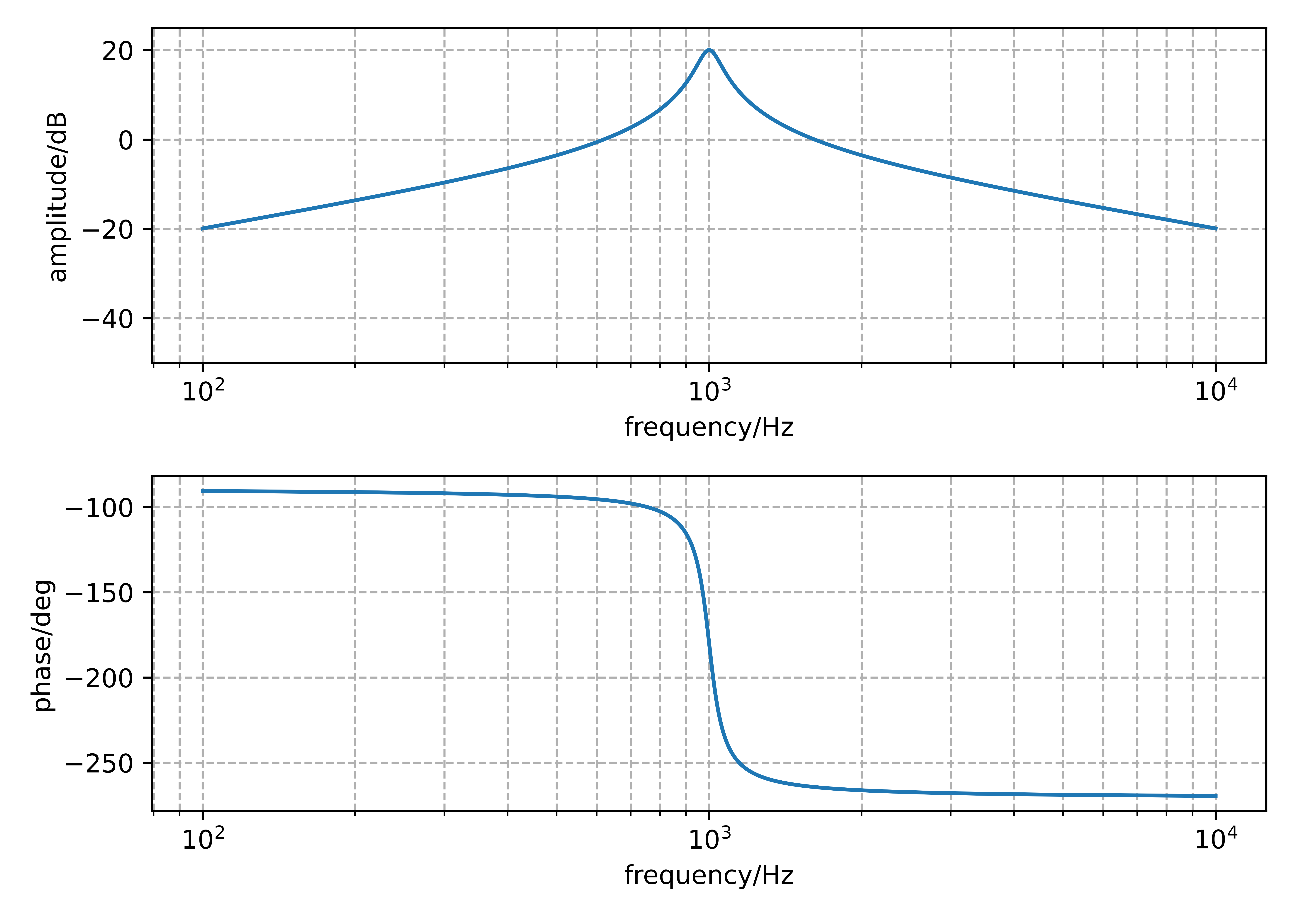

Figure 3.3: Frequency response of the band pass filter

Band stop

The output for the band stop filter is marked in Figure 2.1 as \(BSF\) and in the transfer function as \(V_{04}\).

\[ \frac{V_{04}}{V_i} = \frac{\left( 1 + \frac{s^2}{\omega_0^2} \right) \cdot H_0}{\left( 1 + \frac{s}{\omega_0 Q} + \frac{s^2}{\omega_0^2} \right)} \tag{3.4}\]

(Renner 2025) argues that Equation 3.4 from the ASLK PRO Manual (Rao and Ravikumar 2012) is incorrect, as using that equation produces inconsistent results. Using the negated form of Equation 3.4 as seen in Equation 3.5 seems to produce the correct output. Therefore Equation 3.5 will be used for further analysis.

\[ \frac{V_{04}}{V_i} = - \frac{\left( 1 + \frac{s^2}{\omega_0^2} \right) \cdot H_0}{\left( 1 + \frac{s}{\omega_0 Q} + \frac{s^2}{\omega_0^2} \right)} \tag{3.5}\]

Figure 3.4 shows the frequency response of the band stop, with its center frequency at \(1\,kHz\).

Listing 3.4

# Behavioral Analysis Biquad Filter

import numpy as np
import matplotlib.pyplot as plt

# Initial values
f0 = 1e3  # Resonance frequency in Hz
w0 = 2 * np.pi * f0  # Angular frequency in rad/s
Q = 10  # Quality factor
H0 = 1  # Play around with this later

# Logarithmic frequency axis
frequencies = np.logspace(2, 4, 10000)  # Frequency from 10^2 to 10^4 Hz
s = 1j * 2 * np.pi * frequencies  # Laplace-Variable s = jω

############################################
# Transfer functions of Active Filters
############################################

### Numerator
# Low Pass Filter
b_lp = H0

# High Pass Filter
b_hp = (H0 * (s**2 / w0**2))

# Band Pass Filter
b_bp = (-H0 * (s / w0))

# Band Stop Filter
b_bs = -((1 + (s**2 / (w0**2))) * H0)

# Denominator -> for all filters the same
a0 = 1
a1 = (s / (w0 * Q))
a2 = (s**2 / (w0**2))

den = a0 + a1 + a2

############################################
# Calculation of the transfer functions H(s)
############################################
Hs_lp = b_lp / den
Hs_hp = b_hp / den
Hs_bp = b_bp / den
Hs_bs = b_bs / den

# Bode Diagram
fig, axs = plt.subplots(2)
#fig.suptitle("frequency response of biquad filter")
'''
# Low Pass Filter
axs[0].semilogx(frequencies, 20 * np.log10(np.abs(Hs_lp)), label='low pass')
axs[1].semilogx(frequencies, np.unwrap(np.angle(Hs_lp)) * (180 / np.pi), label='low pass')

# High Pass Filter
axs[0].semilogx(frequencies, 20 * np.log10(np.abs(Hs_hp)), label='high pass')
axs[1].semilogx(frequencies, np.unwrap(np.angle(Hs_hp)) * (180 / np.pi), label='high pass')

# Band Pass Filter
axs[0].semilogx(frequencies, 20 * np.log10(np.abs(Hs_bp)), label='band pass')
axs[1].semilogx(frequencies, np.unwrap(np.angle(Hs_bp)) * (180 / np.pi), label='band pass')
'''
# Band Stop Filter
axs[0].semilogx(frequencies, 20 * np.log10(np.abs(Hs_bs)), label='band stop')
axs[1].semilogx(frequencies, (np.angle(Hs_bs)) * (180 / np.pi), label='band stop')

#axs[0].title("amplitude response")
axs[0].set_xlabel("frequency/Hz")
axs[0].set_ylabel("amplitude/dB")
axs[0].set_ylim(-50, 25)
axs[0].grid(True, which="both", ls="--")
#axs[0].legend(loc=1)

#axs[1].title("phase response")
axs[1].set_xlabel("frequency/Hz")
axs[1].set_ylabel("phase/deg")
axs[1].grid(True, which="both", ls="--")
#axs[1].legend()

plt.tight_layout()
#plt.show()

plt.savefig("../images/sec_characterisation/freqResponseBandstop.png", format="png", dpi=1000)

Figure 3.4: Frequency response of the band stop filter

Comparison

Figure 3.5 shows all four frequency responses together in oen graph. It shows nicely that all three pass filters peak at the same freqeuncy and the same height. Comparing this plot with the one from (Rao and Ravikumar 2012) gives reason to argue that the filter design on a theoretic system level should work.

Listing 3.5

# Behavioral Analysis Biquad Filter

import numpy as np
import matplotlib.pyplot as plt

# Initial values
f0 = 1e3  # Resonance frequency in Hz
w0 = 2 * np.pi * f0  # Angular frequency in rad/s
Q = 10  # Quality factor
H0 = 1  # Play around with this later

# Logarithmic frequency axis
frequencies = np.logspace(2, 4, 10000)  # Frequency from 10^2 to 10^4 Hz
s = 1j * 2 * np.pi * frequencies  # Laplace-Variable s = jω

############################################
# Transfer functions of Active Filters
############################################

### Numerator
# Low Pass Filter
b_lp = H0

# High Pass Filter
b_hp = (H0 * (s**2 / w0**2))

# Band Pass Filter
b_bp = (-H0 * (s / w0))

# Band Stop Filter
b_bs = -((1 + (s**2 / (w0**2))) * H0)

# Denominator -> for all filters the same
a0 = 1
a1 = (s / (w0 * Q))
a2 = (s**2 / (w0**2))

den = a0 + a1 + a2

############################################
# Calculation of the transfer functions H(s)
############################################
Hs_lp = b_lp / den
Hs_hp = b_hp / den
Hs_bp = b_bp / den
Hs_bs = b_bs / den

# Bode Diagram
fig, axs = plt.subplots(2)
#fig.suptitle("frequency response of biquad filter")

# Low Pass Filter
axs[0].semilogx(frequencies, 20 * np.log10(np.abs(Hs_lp)), label='low pass')
axs[1].semilogx(frequencies, np.unwrap(np.angle(Hs_lp)) * (180 / np.pi), label='low pass')

# High Pass Filter
axs[0].semilogx(frequencies, 20 * np.log10(np.abs(Hs_hp)), label='high pass')
axs[1].semilogx(frequencies, np.unwrap(np.angle(Hs_hp)) * (180 / np.pi), label='high pass')

# Band Pass Filter
axs[0].semilogx(frequencies, 20 * np.log10(np.abs(Hs_bp)), label='band pass')
axs[1].semilogx(frequencies, np.unwrap(np.angle(Hs_bp)) * (180 / np.pi), label='band pass')

# Band Stop Filter
axs[0].semilogx(frequencies, 20 * np.log10(np.abs(Hs_bs)), label='band stop')
axs[1].semilogx(frequencies, (np.angle(Hs_bs)) * (180 / np.pi), label='band stop')

#axs[0].title("amplitude response")
axs[0].set_xlabel("frequency/Hz")
axs[0].set_ylabel("amplitude/dB")
axs[0].set_ylim(-50, 25)
axs[0].grid(True, which="both", ls="--")
axs[0].legend(loc=1)

#axs[1].title("phase response")
axs[1].set_xlabel("frequency/Hz")
axs[1].set_ylabel("phase/deg")
axs[1].grid(True, which="both", ls="--")
axs[1].legend()

plt.tight_layout()
#plt.show()

plt.savefig("../images/sec_characterisation/freqResponseFilter.png", format="png", dpi=1000)

Figure 3.5: Behauvioural analysis of biquad filter

3.1.2 Stability

The stability of the biquad is checked at different hierarchical levels. The first analysis considers the system from a theorectical standpoint with transfer functions, and checks if conceptual design of the biquad filter is stable. On a component level the stability of the integrators and adders is analyzed, to verify that the chosen values for resistors and capcitors do not induce oscillations through the feedback loop.

3.1.2.1 System stability

A system is stable if its impulse response is absolutley integrateable. In case of a given transfer function, this can also be checked by calculating the poles of the transfer function. If all the poles lay in the left half of the s-plane, the system is considered stable. There is a special case where single poles can lay on the \(j\omega\)-axis, on their own or in combination with poles in the left half of the s-plane. Systems which fall under that, are called marginally stable. (Fliege 1991)

3.1.2.2 Pole-zero plot

Listing 3.6

import numpy as np
import matplotlib.pyplot as plt
from scipy.signal import tf2zpk

# Given values
f = 1e3
w = 2 * np.pi * f
R = 1e3
C = 1 / (w * R)
Q = 10
H0 = 1

# Calculate w0
w0 = 1 / (R * C)

# Transfer function coefficients
a2 = 1 / w0**2
a1 = 1 / (w0 * Q)
a0 = 1

# Define transfer functions manually as (numerator, denominator) pairs
systems = {
    'Low pass filter': ([H0], [a2, a1, a0]),
    'High pass filter': ([H0 / w0**2, 0, 0], [a2, a1, a0]),
    'Band pass filter': ([-H0 / w0, 0], [a2, a1, a0]),
    'Band stop filter': ([H0 / w0**2, 0, H0], [a2, a1, a0])
}

# Function to plot pole-zero map
def plot_pzmap(num, den, title, subplot_pos):
    zeros, poles, _ = tf2zpk(num, den)
    plt.subplot(2, 2, subplot_pos)
    plt.plot(np.real(zeros), np.imag(zeros), 'go', label='Zeros')
    plt.plot(np.real(poles), np.imag(poles), 'rx', label='Poles')
    plt.axhline(0, color='gray', lw=0.5)
    plt.axvline(0, color='gray', lw=0.5)
    plt.title(title)
    plt.xlabel('$\sigma$')
    plt.ylabel('$j\omega$')
    plt.xlim([-1500, 1500])
    plt.ylim([-10000, 10000])
    plt.grid(True)
    plt.legend(loc='upper right')

# Plot all systems
plt.figure(figsize=(12, 10))
for i, (title, (num, den)) in enumerate(systems.items(), 1):
    plot_pzmap(num, den, title, i)

plt.tight_layout()
#plt.show()

plt.savefig("../images/sec_characterisation/poleZeroStability.png", format="png", dpi=1000)

Figure 3.6: Pole-zero plot for all transfer functions

Figure 3.6 shows the pole-zero plots of all four filters, low pass, high pass, band pass and band stop. In all four plots the poles are located in the left half of the s-plane and the system can therefore theoretically be classified as stable. (Razavi 2018) confirms this, as the article explains that with \(Q \rightarrow \infty\) the poles of the system approach the \(j\omega\) axis and the system becomes unstable.

This analysis only considers the system as a mathematical model and as a whole. Further considerations regarding the stability of the components, integrators and adders, have to be done.

3.1.2.3 Component stability

Circuits with opamps often have feedback loops, meaning that the output of the operational amplifier is somehow connected to the inverted input of the opamp. These feedback loops become problematic when the feedback signal is in phase with the input signal, as positive feedback is created and the circuit is working as an oscillator. (Reisch 2007)

The stability of the non-inverting amplifier can be verified by calculating the phase reserve \(\alpha\) of the circuit. If \(f_k\) is the frequency where the feedback gain is equal to 1 and \(\varphi_k\) is the corresponding phase to that frequency, then the phase reserve is calculated by:

\[ \alpha = 180° - \varphi_k \]

For circuits to be considered stable, the phase reserve has to be positive. To reduce overshoots during the transient response, it is customary to have a phase reserve of \(\alpha > 45°\). (Reisch 2007)

Figure 3.7: Example of a transcient response of a circuit with a phase reserve of \(\alpha = 5.7°\) (taken from Reisch 2007)

Figure Figure 3.7 shows the transient response of a circuit with a phase reserve of \(\alpha = 5.7°\). The overshoots are clearly visible and number of the overshoots per puls are larger then the customary “one over, one under”-rule. As the phase reserve is positive, the figure shows that even though the transient response is not ideal, the oscillations are attenuated and the circuit is can be considered as stable.

In practical application, the phase reserve can be graphically determined with the help of bode diagrams. The bode diagram of the circuit with an open feedback loop is simulated, so that the frequency \(f_k\) can be read out. This is the frequency where the feedback gain is 1 or 0 dB. The corresponding frequency to that, is the phase of the feedback gain \(\varphi_k\), the difference between \(-180°\) and \(\varphi_k\) is the phase reserve \(\alpha\). (Reisch 2007)

For the analysis of component stability the 5t-ota design from (Pretl, Koefinger, and Dorrer 2025) was used. Figure 3.8 and Figure 3.9 show the schematics that simulated the stability analysis for the components. In both cases the AC source was inserted in the open feedback loop and the output of the OTA was used to analyse the stability.

Figure 3.8: Circuit schematic of the stability analysis of the adder

Figure 3.9: Circuit schematic of the stability analysis of the integrator

In the following figures Figure 3.10 and Figure 3.11 this stability analysis method was used to determine the stability over the phase reserve.

Listing 3.7

# Stability analysis adder

import numpy as np
import matplotlib.pyplot as plt
import sys
sys.path.insert(0, '../simulation')
import ltspy3

sd=ltspy3.SimData('../simulation/stability_adder.raw',[b'v(v_out)',b'frequency'])

nvout = sd.variables.index(b'v(v_out)')
nfrequency = sd.variables.index(b'frequency')

fig, (ax1, ax2) = plt.subplots(2, 1, figsize=(10, 6), sharex=True)

ax1.semilogx(sd.values[nfrequency],20*np.log10(abs(sd.values[nvout])))
ax1.set_ylabel("Magnitude/dB")
ax1.axvline(3e5,color='red',linestyle='--')
ax1.grid(True, which="both", ls="--")

ax2.semilogx(sd.values[nfrequency],np.angle(sd.values[nvout], deg=True))
ax2.axvline(3e5,color='red',linestyle='--')
ax2.axhline(82.75,color='red',linestyle='--')
ax2.set_ylabel("Phase/deg")
ax2.set_xlabel("Frequency/Hz")


plt.grid(True, which="both", ls="--")
plt.tight_layout()
#plt.show()

plt.savefig("../images/sec_characterisation/stabilityAdder.png", format="png", dpi=1000)

Figure 3.10: Stability analysis of the adder

The frequency response of the adder shows a phase \(\varphi_k = 83°\), when the gain is 1. Calculation the phase reserve from that

\[\alpha_{add} = 180° - \varphi_k = 180° - 83° = 97° > 45° \]

gives a phase reserves, that indicates stability for this component.

Listing 3.8

# Stability analysis integrator

import numpy as np
import matplotlib.pyplot as plt
import sys
sys.path.insert(0, '../simulation')
import ltspy3

sd=ltspy3.SimData('../simulation/stability_integrator.raw',[b'v(v_out)',b'frequency'])

nvout = sd.variables.index(b'v(v_out)')
nfrequency = sd.variables.index(b'frequency')

fig, (ax1, ax2) = plt.subplots(2, 1, figsize=(10, 6), sharex=True)

ax1.semilogx(sd.values[nfrequency],20*np.log10(abs(sd.values[nvout])))
ax1.set_ylabel("Magnitude/dB")
ax1.axvline(7e5,color='red',linestyle='--')
ax1.grid(True, which="both", ls="--")

ax2.semilogx(sd.values[nfrequency],np.angle(sd.values[nvout], deg=True))
ax2.axvline(7e5,color='red',linestyle='--')
ax2.axhline(68,color='red',linestyle='--')
ax2.set_ylabel("Phase/deg")
ax2.set_xlabel("Frequency/Hz")

plt.grid(True, which="both", ls="--")
plt.tight_layout()
#plt.show()

plt.savefig("../images/sec_characterisation/stabilityIntegrator.png", format="png", dpi=1000)

Figure 3.11: Stability analysis of the integrator

The stability of the integrator circuit, as seen in Figure 3.11, shows a intersection of the magnitude plot with the \(0\,dB\) line at about \(f_k = 70\,kHz\), which corresponds to a phase of \(\varphi_k = 68°\). This would leave a phase reserve of:

\[ \alpha_{int} = 180° - \varphi_k = 112° > 45° \]

Therefore the integrator would be stable.

3.1.3 Ideal Opamp

To check the behauviour of the implemented circuit against the modelled behauviour of the transfer function, the universal biquad was built as an ideal circuit with voltage-regulated current sources instead of OTAs. This simulation of the circuit verfies that the circuit implementation of the biquadratic filter with OTAs can fulfill the requirements at least in the ideal case.

Figure 3.12: Schematic of an universal biquad filter with ideal OTAs

Figure 3.12 depicts the schematic of an universal biquad filter, where the OTAs are idealised with voltage controlled current sources. An ac simulation of this circuit can be viewed in Figure 3.13.

Listing 3.9

# plot Ideal (voltage controlled current? source) biquad
import numpy as np
import matplotlib.pyplot as plt
import sys
sys.path.insert(0, '../simulation')
import ltspy3

sd=ltspy3.SimData('../simulation/biquad_univ.raw')

nvoutLPF = sd.variables.index(b'v(lpf)')
nvoutHPF = sd.variables.index(b'v(hpf)')
nvoutBPF = sd.variables.index(b'v(bpf)')
nvoutBSF = sd.variables.index(b'v(bsf)')
nfrequency = sd.variables.index(b'frequency')

fig, (ax1, ax2) = plt.subplots(2, 1, figsize=(10, 6), sharex=True)

ax1.semilogx(sd.values[nfrequency],20*np.log10(abs(sd.values[nvoutLPF])),label='lpf')
ax1.semilogx(sd.values[nfrequency],20*np.log10(abs(sd.values[nvoutHPF])),label='hpf')
ax1.semilogx(sd.values[nfrequency],20*np.log10(abs(sd.values[nvoutBPF])),label='bpf')
ax1.semilogx(sd.values[nfrequency],20*np.log10(abs(sd.values[nvoutBSF])),label='bsf')
ax1.set_xlim([10e1,10e3])
ax1.set_ylim([-40,20])
ax1.set_ylabel("Magnitude/dB")
ax1.grid(True, which="both", ls="--")
ax1.legend()

ax2.semilogx(sd.values[nfrequency],np.angle(sd.values[nvoutLPF], deg=True),label='lpf')
ax2.semilogx(sd.values[nfrequency],np.angle(sd.values[nvoutHPF], deg=True),label='hpf')
ax2.semilogx(sd.values[nfrequency],np.angle(sd.values[nvoutBPF], deg=True),label='bpf')
ax2.semilogx(sd.values[nfrequency],np.angle(sd.values[nvoutBSF], deg=True),label='bsf')
ax2.set_ylabel("Phase/deg")
ax2.set_xlabel("Frequency/Hz")
ax2.legend()

plt.grid(True, which="both", ls="--")
plt.tight_layout()
#plt.show()

plt.savefig("../images/sec_characterisation/idealCir.png", format="png", dpi=1000)

Figure 3.13: Simulation of an idealised biquad

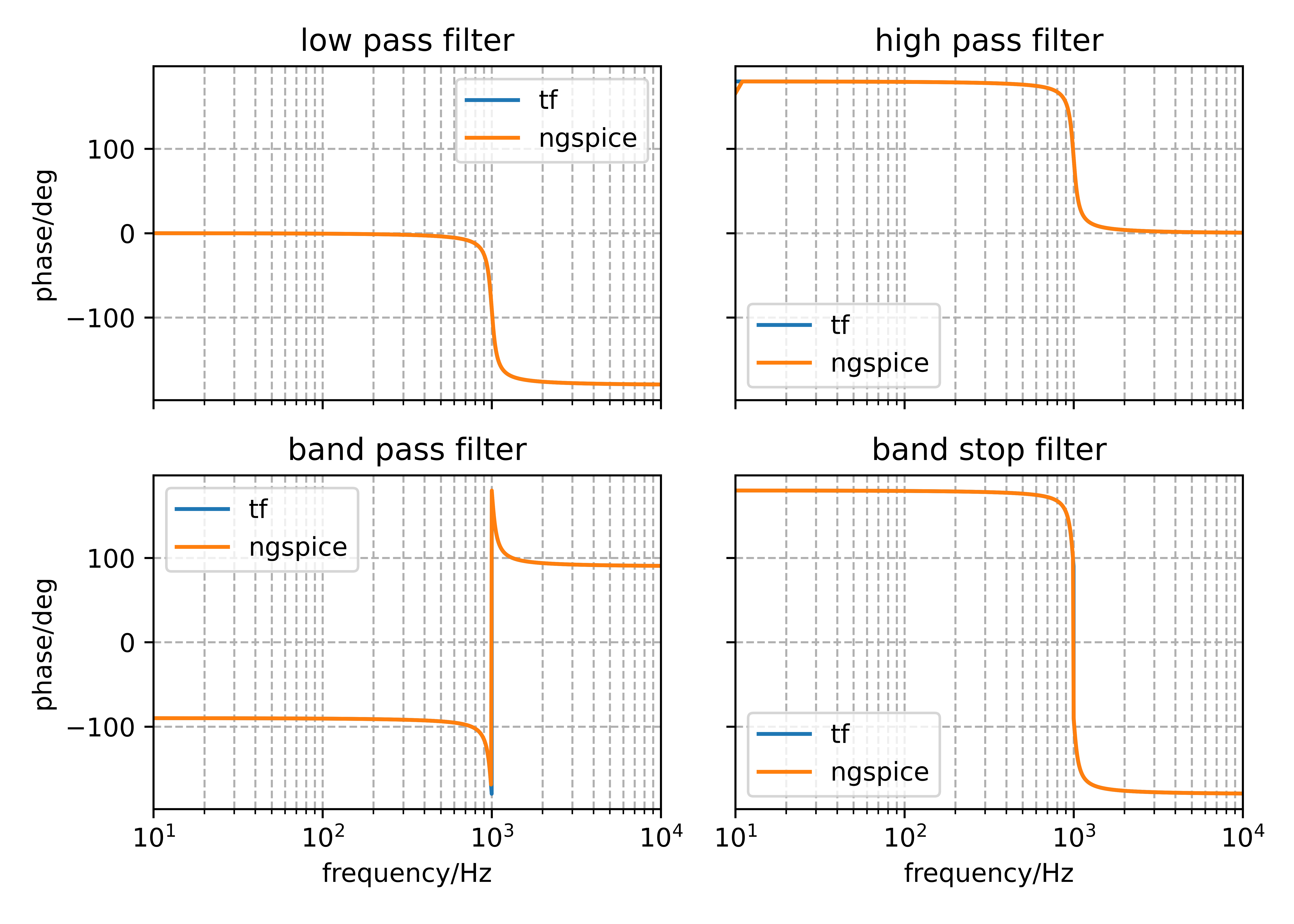
Figure 3.14 and Figure 3.15 compares the system-theoretic analysis with transfer functions with the simulated idealised of the filter design with each other. Both plots show very nicely that the amplitude response as well as the phase response of all four filters match with their simulated and calculated responses.

Listing 3.10

import numpy as np
import matplotlib.pyplot as plt
import sys
sys.path.insert(0, '../simulation')
import ltspy3

sd=ltspy3.SimData('../simulation/biquad_univ.raw')

nvoutLPF = sd.variables.index(b'v(lpf)')
nvoutHPF = sd.variables.index(b'v(hpf)')
nvoutBPF = sd.variables.index(b'v(bpf)')
nvoutBSF = sd.variables.index(b'v(bsf)')
nfrequency = sd.variables.index(b'frequency')

#behauvioural moddling with tfs

# Initial values
f0 = 1000  # Resonance frequency in Hz
w0 = 2 * np.pi * f0  # Angular frequency in rad/s
Q = 10  # Quality factor
H0 = 1  # Play around with this later

# Logarithmic frequency axis
frequencies = np.logspace(0, 5, 10000)  # Frequency from 10^2 to 10^4 Hz
s = 1j * 2 * np.pi * frequencies  # Laplace-Variable s = jω

############################################
# Transfer functions of Active Filters
############################################


### Numerator
# Low Pass Filter
b_lp = H0

# High Pass Filter
b_hp = (H0 * (s**2 / w0**2))

# Band Pass Filter
b_bp = (-H0 * (s / w0))

# Band Stop Filter
b_bs = -(1 + (s**2 / (w0**2))) * H0

# Denominator -> for all filters the same
a0 = 1
a1 = (s / (w0 * Q))
a2 = (s**2 / (w0**2))

den = a0 + a1 + a2

############################################
# Calculation of the transfer functions H(s)
############################################
Hs_lp = b_lp / den
Hs_hp = b_hp / den
Hs_bp = b_bp / den
Hs_bs = b_bs / den

#mag plots

fig, axs = plt.subplots(2, 2, sharex=True, sharey=True)

ax1, ax2, ax3, ax4 = axs.flatten()

# Plotting each
ax1.semilogx(frequencies, 20 * np.log10(np.abs(Hs_lp)), label='tf')
ax1.semilogx(sd.values[nfrequency], 20 * np.log10(abs(sd.values[nvoutLPF])), label='ngspice')
ax1.set_ylabel("magnitude/dB")
ax1.set_title("low pass filter")
ax1.set_xlim([10,10e4])
ax1.set_ylim([-60,25])
ax1.grid(True, which="both", ls="--")
ax1.legend()

ax2.semilogx(frequencies, 20 * np.log10(np.abs(Hs_hp)), label='tf')
ax2.semilogx(sd.values[nfrequency], 20 * np.log10(abs(sd.values[nvoutHPF])), label='ngspice')
ax2.set_title("high pass filter")
#ax2.set_xlim([10,10e3])
#ax2.set_ylim([-40,25])
ax2.grid(True, which="both", ls="--")
ax2.legend()

ax3.semilogx(frequencies, 20 * np.log10(np.abs(Hs_bp)), label='tf')
ax3.semilogx(sd.values[nfrequency], 20 * np.log10(abs(sd.values[nvoutBPF])), label='ngspice')
ax3.set_xlabel("frequency/Hz")
ax3.set_ylabel("magnitude/dB")
ax3.set_title("band pass filter")
#ax3.set_xlim([10,10e3])
#ax3.set_ylim([-40,25])
ax3.grid(True, which="both", ls="--")
ax3.legend()

ax4.semilogx(frequencies, 20 * np.log10(np.abs(Hs_bs)), label='tf')
ax4.semilogx(sd.values[nfrequency], 20 * np.log10(abs(sd.values[nvoutBSF])), label='ngspice')
ax4.set_xlabel("frequency/Hz")
ax4.set_title("band stop filter")
#ax4.set_xlim([10,10e3])
#ax4.set_ylim([-40,25])
ax4.grid(True, which="both", ls="--")
ax4.legend()

plt.tight_layout()
#plt.show()

plt.savefig("../images/sec_characterisation/compTfIdealAmplitude.png", format="png", dpi=1000)

Figure 3.14: Comparison of the amplitude response between the transfer functions and idealised circuit

Listing 3.11

import numpy as np
import matplotlib.pyplot as plt
import sys
sys.path.insert(0, '../simulation')
import ltspy3

sd=ltspy3.SimData('../simulation/biquad_univ.raw')

nvoutLPF = sd.variables.index(b'v(lpf)')
nvoutHPF = sd.variables.index(b'v(hpf)')
nvoutBPF = sd.variables.index(b'v(bpf)')
nvoutBSF = sd.variables.index(b'v(bsf)')
nfrequency = sd.variables.index(b'frequency')

#behauvioural moddling with tfs

# Initial values
f0 = 1000  # Resonance frequency in Hz
w0 = 2 * np.pi * f0  # Angular frequency in rad/s
Q = 10  # Quality factor
H0 = 1  # Play around with this later

# Logarithmic frequency axis
frequencies = np.logspace(0, 4, 10000)  # Frequency from 10^2 to 10^4 Hz
s = 1j * 2 * np.pi * frequencies  # Laplace-Variable s = jω

############################################
# Transfer functions of Active Filters
############################################


### Numerator
# Low Pass Filter
b_lp = H0

# High Pass Filter
b_hp = (H0 * (s**2 / w0**2))

# Band Pass Filter
b_bp = (-H0 * (s / w0))

# Band Stop Filter
b_bs = -(1 + (s**2 / (w0**2))) * H0

# Denominator -> for all filters the same
a0 = 1
a1 = (s / (w0 * Q))
a2 = (s**2 / (w0**2))

den = a0 + a1 + a2

############################################
# Calculation of the transfer functions H(s)
############################################
Hs_lp = b_lp / den
Hs_hp = b_hp / den
Hs_bp = b_bp / den
Hs_bs = b_bs / den

#phase plots

fig, axs = plt.subplots(2, 2, sharex=True, sharey=True)

ax1, ax2, ax3, ax4 = axs.flatten()

# Plotting each
ax1.semilogx(frequencies, np.angle(Hs_lp, deg=True), label='tf')
ax1.semilogx(sd.values[nfrequency],np.angle(sd.values[nvoutLPF], deg=True),label='ngspice')
ax1.set_ylabel("phase/deg")
ax1.set_title("low pass filter")
ax1.set_xlim([10,10e3])
#ax1.set_ylim([-40,25])
ax1.grid(True, which="both", ls="--")
ax1.legend()

ax2.semilogx(frequencies, np.angle(Hs_hp, deg=True), label='tf')
ax2.semilogx(sd.values[nfrequency],np.angle(sd.values[nvoutHPF], deg=True),label='ngspice')
ax2.set_title("high pass filter")
#ax1.set_xlim([10,10e3])
#ax1.set_ylim([-40,25])
ax2.grid(True, which="both", ls="--")
ax2.legend()

ax3.semilogx(frequencies, np.angle(Hs_bp, deg=True), label='tf')
ax3.semilogx(sd.values[nfrequency],np.angle(sd.values[nvoutBPF], deg=True),label='ngspice')
ax3.set_xlabel("frequency/Hz")
ax3.set_ylabel("phase/deg")
ax3.set_title("band pass filter")
#ax1.set_xlim([10,10e3])
#ax1.set_ylim([-40,25])
ax3.grid(True, which="both", ls="--")
ax3.legend()

ax4.semilogx(frequencies, np.angle(Hs_bs, deg=True), label='tf')
ax4.semilogx(sd.values[nfrequency],np.angle(sd.values[nvoutBSF], deg=True),label='ngspice')
ax4.set_xlabel("frequency/Hz")
ax4.set_title("band stop filter")
#ax1.set_xlim([10,10e3])
#ax1.set_ylim([-40,25])
ax4.grid(True, which="both", ls="--")
ax4.legend()

plt.tight_layout()
#plt.show()

plt.savefig("../images/sec_characterisation/compTfIdealPhase.png", format="png", dpi=1000)

Figure 3.15: Comparison of the phase response between the transfer functions and idealised circuit

Fliege, Norbert. 1991. Systhemtheorie. 1st ed. Stuttgart: Teubner.

Pretl, Harald, Michael Koefinger, and Simon Dorrer. 2025. “Analog Circuit Design.” https://doi.org/10.5281/zenodo.14387481.

Rao, K. R. K., and C. P. Ravikumar. 2012. Analog System Lab Kit PRO MANUAL. Texas Instruments.

Razavi, Behzad. 2018. “The Biquadratic Filter.” IEEE Solid-State Circuit Magazine, 11–16.

Reisch, Michael. 2007. Elektronische Bauelemente - Funktion, Grundschaltungen, Modellierung Mit SPICE. 2nd ed. Stuttgart: Springer-Verlag.

Renner, Nils. 2025. “Biquadratic IIR (SOS) Filters.”